SETS, RELATIONS AND FUNCTIONS:
INTRODUCTION
The concepts of sets, relations and functions occupy a
fundamental place in the mainstream of mathematical thinking. As rightly stated
by the Russian mathematician Luzin the concept of
functions did not arise suddenly. It underwent profound changes in time.
Galileo (1564-1642) explicitly used the dependency of one quantity on another
in the study of planetary motions. Descartes (1596-1650) clearly stated that an
equation in two variables, geometrically represented by a curve, indicates
dependence between variable quantities
SETS
In the earlier classes, we have seen that a set is a collection of
well-defined objects. As the theory of sets is the building blocks of modern mathematics,
one has to learn the concepts of sets carefully and deeply. Now we look at the
term “well-defined” a little more deeply. Consider the two statements:
![]() The collection of all beautiful
flowers in Ooty Rose Garden.
The collection of all beautiful
flowers in Ooty Rose Garden.
![]() The collection of all old men
in Tamilnadu.
The collection of all old men
in Tamilnadu.
The terms “beautiful flowers” and “old men” are not
well-defined. We cannot define the term “beautiful flower” in a sharp way as
there is no concrete definition for beauty because the concept of beauty varies
from person to person, content to content and object to object. We should not
consider statements like “the collection of all beautiful flowers in Ooty Rose Garden” as a set. Now, can we say “the collection
of all red flowers in Ooty Rose Garden” a set? The
answer is “yes”.
We have also seen and learnt to use symbols like ∈, ᑕ, U and ∩. Let us start with the question:
“ If A and B are
two sets, is it meaningful to write A ∈ B?”.
At the first sight one may hurry to say that this is always
meaningless by telling, “the symbol ∈ should
be used between an element and a set and it should not be used between two
sets”. The first part of the statement is true whereas the second part is not
true. For example, if A = {1, 2} and = {1, {1, 2}, 3, 4},
then A ∈ B. In this section we shall discuss the meaning of
such symbols more deeply.
As we learnt in the earlier classes the set containing no
elements is called an empty set or a void set. It is usually denoted by Ø or { }. By ![]() ,
we mean every element of the set A is an element of the set B. In this case, we say A is
a subset of B and B is
a super set of A.
For any two sets A and B , if
,
we mean every element of the set A is an element of the set B. In this case, we say A is
a subset of B and B is
a super set of A.
For any two sets A and B , if ![]() , then the two sets are equal. For any set A,
the empty set Ø and the set A are always subsets of A.
These two subsets are called trivial subsets
, then the two sets are equal. For any set A,
the empty set Ø and the set A are always subsets of A.
These two subsets are called trivial subsets
We learnt that the union of two sets A and B is
denoted by A U B and is defined as
A U B = {x : x ∈ A or x ∈ B}
and the intersection as
A ∩ B = {x : x ∈ A and x ∈ B}.
Two sets A and B are disjoint if they do not have
any common element. That is, A and B are
disjoint if A ∩ B = ∅.

PROPERTIES OF SET OPERATIONS
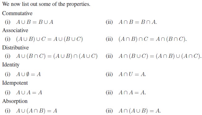
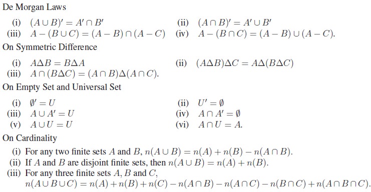
CARTESIAN
PRODUCT
We know that the Cartesian product of sets is nothing but a set
of ordered elements. In particular, Cartesian product of two sets is a set of
ordered pairs, while the Cartesian product of three sets is a set of ordered
triplets. Precisely, let A, B and C be three
non-empty sets. Then the Cartesian product of A with B is denoted
by A × B. It is
defined by
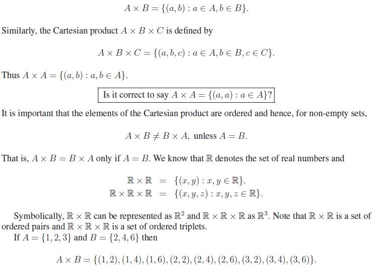
Here A × B is
a subset of R × R. The number of elements
in A × B is the product of the number
of elements in A and the number of elements in B,
that is, n(A × B) = n(A)n(B),
if A and B are finite. Further n(A × B × C)
= n(A)n(B)n(C), if A, B and C are
finite.
It is easy to see that the following are the subsets
of R × R.

1.
If A={x:x=4n+1,2≤n≤5}, then number of subsets of
ANSWER
A={X:x=4n+12≤n≤5}
⇒A={4(2)+1,4(3)+1,4(4)+1,4(5)+1}
⇒2{9,13,17,21}
no of subsets of A=24=16
2. In a survey of 5000 persons in a
town, it was found that 45% of the persons know language a, 25% know language
b, 10% know language c, 5% know languages a and b, 4% know languages b and c,
and 4% know languages a and
c. if 3% of the persons know all the three languages, find the number of
persons who knows only language
Those who know language a = 45%
x 5000
= 2250
Those who know language b = 25%
x 5000
= 1250
Those who know languages a and b
= 5% x 5000
= 250
Those who know a alone = 2250 -
250
= 2000
CONSTANTS
AND VARIABLES, INTERVALS AND NEIGHBOURHOODS
To continue our discussion, we need certain prerequisites
namely, constants, variables, independent variables, dependent variables,
intervals and neighbourhoods.
1. CONSTANTS AND VARIABLES
A quantity that remains unaltered throughout a
mathematical process is called a constant.
A quantity that varies in a mathematical process is called a variable.
A variable is an independent variable when
it takes any arbitrary (independent) value not depending on any other
variables, whereas if its value depends on other variables, then it is called
a dependent variable.
We know the area A of a triangle is given
by A = 1/2 bh.
Here 1/2 is a constant and A, b, h are variables.
Moreover b and h are independent variables
and A is a dependent variable. We ought to note that the
terms dependent and independent are relative
terms. For example in the equation x + y =
1, x, y are variables and 1 is a
constant. Which of x and y is dependent and
which one is independent? If we consider x as an
independent variable, then y becomes a dependent whereas if we
consider y as an independent variable, then x becomes
dependent.
Further consider the following examples:
![]() area
of a rectangle A = lb.
area
of a rectangle A = lb.
![]() area
of a circle A = πr2.
area
of a circle A = πr2.
![]() volume
of a cuboid V = lbh.
volume
of a cuboid V = lbh.
From the above examples we can directly infer that b, h,
l , r are independent variables; A and V are
dependent variables and π is a constant .
2.
INTERVALS AND NEIGHBOURHOODS
The system R of real numbers can be
represented by the points on a line and a point on the line can be related to a
unique real number as in Figure 1.2. By this, we mean that any real number can
be identified as a point on the line. With this identification we call the line
as the real line.

The value increases as we go right and decreases as we go left.
If x lies to the left of y on the real line
then x < y. As there is no gap in a line, we have infinitely
many real numbers between any two real numbers.
![]() The set of all real numbers greater than 0.
The set of all real numbers greater than 0.
![]() The set of all real numbers
greater than 5 and less than 7.
The set of all real numbers
greater than 5 and less than 7.
![]() The set of all real
numbers x such that 1 ≤ x ≤ 3.
The set of all real
numbers x such that 1 ≤ x ≤ 3.
![]() The set of all real
numbers x such that 1 < x ≤ 2.
The set of all real
numbers x such that 1 < x ≤ 2.
The above four sets are
intervals. In particular (i) is an infinite interval
and (ii), (iii) and (iv) are finite intervals. The
term “finite interval” does not mean that the interval contains only finitely
many real numbers, however both ends are finite numbers. Both finite and
infinite intervals are infinite sets. The intervals correspond to line segments
are finite intervals whereas the intervals that correspond to rays and the entire
real line are infinite intervals.
A finite interval is said to be closed if it contains both
of its end points and open if it contains neither of its end points. Symbolically the
above four intervals can be written as (0, ∞), (5, 7), [1, 3], (1, 2].
Note that for symbolic form we used parentheses and square brackets to
denote intervals. ( ) parentheses indicate open interval and [
] square brackets indicate closed interval. The first two examples are
open intervals, third one is a closed interval. Note that fourth example is
neither open nor closed, that is, one end open and other end closed.
TYPE OF INTERVALS
There are many types of intervals. Let a, b ∈ R such that a
< b. The following table describes various types of intervals. It is not
possible to draw a line if a point is removed. So we use an unfilled circle “◦”
to indicate that the point is removed and use a filled circle “•” to
indicate that the point is included.
NEIGHBOURHOOD
Neighborhood of
a point ‘a’ is any open interval containing ‘a’. In particular,
if ∈ is a positive number,
usually very small, then the ∈ -neighbourhood
of ‘a’ is the open interval (a − ∈,
a + ∈). The set (a − ∈ ,
a + ∈ ) −
{a} is called deleted neighbourhood of
‘a’ and it is denoted as 0 < |x − a| < ∈ (See
Figure 1.3).

Relations
We approach the concept of relations in different aspects using
real life sense, Cryptography and Geometry through Cartesian products of sets.
In our day to day life very often we come across questions like,
“How is he related to you?”.
Some probable answers are,
![]() He is my father.
He is my father.
![]() He is my teacher.
He is my teacher.
![]() He is not related to me.
He is not related to me.
From this we see that the word relation connects a person with
another person. Extending this idea, in mathematics we consider relations as
one which connects mathematical objects. Examples,
![]() A number m is
related to a number n if m divides n in N.
A number m is
related to a number n if m divides n in N.
![]() A real number x is
related to a real number y if x ≤ y.
A real number x is
related to a real number y if x ≤ y.
![]() A point p is
related to a line L if p lies on L.
A point p is
related to a line L if p lies on L.
![]() A student X is
related to a school S if X is a student
of S.
A student X is
related to a school S if X is a student
of S.
(Cryptography) For centuries, people have used ciphers or codes, to keep confi-dential information secure. Effective ciphers are
essential to the military, to financial institutions and to computer
programmers. The study of the techniques used in creating coding and decoding
these ciphers is called cryptography.
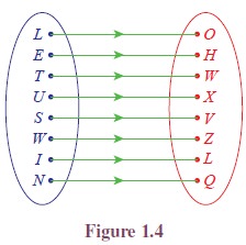
One of the earliest methods of coding a message was a simple
substitution. For example, each letter in a message might be replaced by the
letter that appears three places later in the alphabet.
Using this coding scheme, “LET US WIN” becomes “OHW XVZ LQ”.
This scheme was used by Julius Caesar and is called the Caesars cipher. To
decode, replace each letter by the letter three places before it. This concept
is used often in Mental Ability Tests. The above can be represented as an arrow
diagram as given in Figure 1.4.
This can be viewed as the set of ordered pairs
{(L, O), (E, H), (T, W ), (U,
X), (S, V ), (W, Z), (I,
L), (N, Q)}
which is a subset of the
Cartesian product C × D where C = {L,
E, T, U, S, W, I, N} and D = {O, H, W, X, V,
Z, L, Q}.
Illustration 1.2
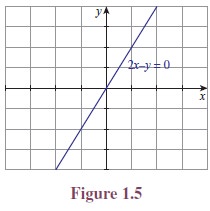
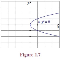
(Geometry) Consider the following three equations
(i) 2x − y = 0
(ii) x2 − y = 0
(iii) x − y2 = 0
(i) 2x − y = 0
The equation 2x − y =
0 represents a straight line. Clearly the points, (1, 2), (3, 6) lie
on it whereas (1, 1), (3, 5), (4, 5) are
not lying on the straight line. The analytical relation between x and y is
given by y = 2x. Here the values of y depends
on the values of x. To denote this dependence, we
write y = f(x). The set of all
points that lie on the straight line is given as {(x, 2x) : x ∈ R}. Clearly this is a subset of R × R. (See
Figure 1.5.)
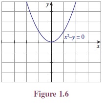
(ii) x2 −
y = 0.
As we discussed earlier, the relation between x and y is y = x2.
The set of all points on the curve is {(x, x2) : x ∈ R} (See
Figure 1.6). Again this is a subset of the Cartesian product RxR.
(iii) x − y2 = 0

From the above examples we intuitively understand what a
relation is. But in mathematics, we have to give a rigorous definition for each
and every technical term we are using. Now let us start defining the term
“relation” mathematically.
Definition of Relation
Let A = {p, q, r, s, t, u} be
a set of students and let B = {X, Y, Z, W } be
a set of schools. Let us consider the following “relation”.
A student a ∈ A is
related to a school S ∈ B if “a”
is studying or studied in the school S.
Let us assume that p studied in X and
now studying in W , q studied
in X and now studying in Y , r studied
in X and W , and now studying in Z, s has
been studying in X from the beginning, t studied in Z and
now studying in no school, and u never studied in any of these
four schools.
Though the relations are given explicitly, it is not possible to
give a relation always in this way. So let us try some other representations
for expressing the same relation:
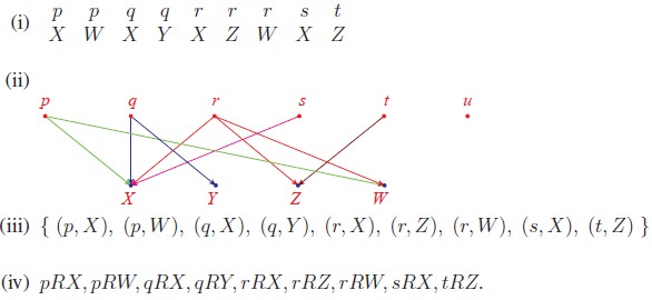
Among these four representations of the relation, the third one
seems to be more convenient and comfortable to deal with a relation in terms of
sets.
The set given in the third representation is a subset of the
Cartesian product A × B.
In Illustrations 1.1 and 1.2 also, we arrived at subsets of a Cartesian
product.
Illustration 1.3 Consider
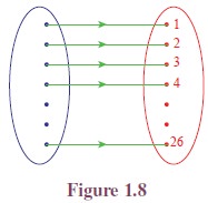
the diagram in Figure 1.8. Here the alphabets are mapped onto the natural numbers.
A simple cipher is to assign a natural number to each alphabet. Here a is
represented by 1, b is represented by 2, . . . , z is represented
by 26. This correspondence can be written as the set of ordered
pairs {(a, 1), (b, 2), . . . , (z, 26)}. This
set of ordered pairs is a relation. The domain of the relation is {a, b, . . . , z} and the range is {1, 2,
. . . , 26}.
Now we recall that the relations discussed in Illustrations 1.1
and 1.2 also end up with subsets of the cartesian
product of two sets. So the term relation used in all
discussions we had so far, fits with the mathematical term relation defined
in Definition 1.2.
The domain of the relation discussed in Illustration 1.1 is the
set {L, E, T, U, S, W, I, N} and the range is {O, H,
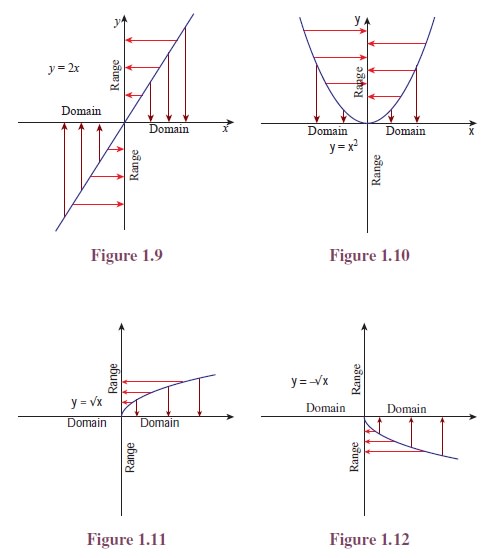
W, X, V, Z, L, Q}. In Illustration 1.2, the domain and range of the
relation discussed for the equation 2x − y =
0 are R and R (See Figure 1.9); for the equation x2 − y =
0, the domain is R and the range is [0, ∞) (See
Figure 1.10); and in the case of the third equation x − y2 =
0, the domain is [0, ∞) and the range
is R (See Figures 1.11 and 1.12).
Note that, the domain of a relation is a subset of the first set
in the Cartesian product and the range is a subset of second set. Usually we
call the second set as co-domain of
the relation. Thus, the range of a relation is the collection of all elements
in the co-domain which are related to some element in the domain. Let us note
that the range of a relation is a subset of the co-domain.
For any set A, Ø and A × A are
subsets of A × A.
These two relations are called extreme
relations.
The former relation is an empty
relation and the later is an universal
relation.
We will discuss more about domain, co-domain and the range in
the next section namely, “Functions”.
If R is a relation from A to B and
if (x, y) ∈ R, then sometimes we write xRy (read this as “x is related
to y”) and if ![]() ,
then sometimes we write x
,
then sometimes we write xRy (read
this as “x is not related to y”).
Though the general definition of a relation is defined from one
set to another set, relations defined on a set are of more interest
in mathematical point of view. That is, relations in which the domain
and the co-domain are the same are of more
interest. So let us concentrate on relations defined on a set.
1. TYPE OF RELATIONS
Consider the following examples:
![]() Let S = {1, 2, 3, 4} and R = {(1, 1), (1, 3), (2, 3)} on S.
Let S = {1, 2, 3, 4} and R = {(1, 1), (1, 3), (2, 3)} on S.
![]() Let S = {1, 2, 3, . . . 10} and define “m is
related to n, if m divides n”.
Let S = {1, 2, 3, . . . 10} and define “m is
related to n, if m divides n”.
![]() Let C be the
set of all circles in a plane and define “a circle C is
related to a circle C , if the radius
of C is equal to the radius of C ”.
Let C be the
set of all circles in a plane and define “a circle C is
related to a circle C , if the radius
of C is equal to the radius of C ”.
![]() In the set S of
all people define “a is related to b,
if a is a brother of b”.
In the set S of
all people define “a is related to b,
if a is a brother of b”.
![]() Let S be
the set of all people. Define the relation on S by the rule
“mother of”.
Let S be
the set of all people. Define the relation on S by the rule
“mother of”.
In the second example, as every number divides itself, “a is related a for all a ∈ S”;
the same is true in the third relation also. In the first example “a is related a for all a ∈ S”
is not true as 2 is not related to 2.
It is easy to see that the property “if a is
related to b, then b is related to a”
is true in the third but not in the second.
It is easy to see that the property “if a is
related to b and b is related to c,
then a is related to c” is true in the second and
third relations but not in the fifth.
These properties, together with some more properties are very
much studied in mathematical structures. Let us define them now.
Let us rewrite the definitions of these basic relations in a
different form:
Let S be any non-empty set. Let R be a relation on S. Then R is
![]() reflexive
if “(a, a) ∈ R for all a ∈ S”.
reflexive
if “(a, a) ∈ R for all a ∈ S”.
![]() symmetric
if “(a, b) ∈ R à (b, a) ∈ R”.
symmetric
if “(a, b) ∈ R à (b, a) ∈ R”.
![]() transitive
if “(a, b), (b, c) ∈ R à (a, c) ∈ R”.
transitive
if “(a, b), (b, c) ∈ R à (a, c) ∈ R”.
Let us consider the following two relations.
In the set S1 of all people,
define a relation R1 by the rule: “a is
related to b, if a is a brother of b”.
In the set S2 of all males,
define a relation R2 by the rule: “a is
related to b, if a is a brother of b”.
The rules that define the relations on S1 and S2 are
the same. But the sets are not same. R1 is not a symmetric
relation on S1 whereas R2 is
a symmetric relation on S2. This shows that not only the
rule defining the relation is important, the set on which the relation is
defined, is also important. So whenever one considers a relation, both the
relation as well as the set on which the relation is defined have to be given
explicitly. Note that the relation {(1, 1), (2, 2), (3, 3), (1, 2)} is
reflexive if it is defined on the set {1, 2, 3};
it is not reflexive if it is defined on the set {1, 2, 3, 4}.
FUNCTIONS
Suppose that a particle is moving in the space. We assume the
physical particle as a point. As time varies, the particle changes its
position. Mathematically at any time the point occupies a position in the three
dimensional space R3. Let us assume that the time varies from 0
to 1. So the movement or functioning of the particle decides
the position of the particle at any given time t between 0 and
1. In other words, for each t ∈ [0, 1],
the functioning of the particle gives a point in R3. Let us
denote the position of the particle at time t as f(t).
A is called the domain of f and B is called the co-domain of f. If (a, b) is in f,
then we write f(a)
= b; the element b is called the image of a and the element a is
called a pre-image of b and f(a) is
known as the value of f at a. The set {b : (a, b) ∈ f for
some a ∈ A} is called the range of the function.
If B is a subset of R, then we say that the function is
a real-valued function.
Two functions f and g are said
to be equal functions if their domains
are same and f(a) = g(a) for
all a in the domain.
If f is a function with domain A and
co-domain B, we write f : A → B (Read
this asf is from A to B or f be
a function from A to B). We also say that f maps A into B.
If f(a) = b, then we
say f maps a to b or a is
mapped onto b by f, and so on.
The range of a function is the collection of all elements in the
co-domain which have pre-images. Clearly the range of a function is a subset of
the co-domain. Further the first condition says that every element in the
domain must have an image; this is the reason for defining the domain of a
relation R from a set A to a set B as
the set of all elements of A having
images and not as A. The second condition says that an
element in the domain cannot have two or more images.
We observe that every function is a relation but a relation need
not be a function.
Let f = {(a, 1), (b, 2), (c, 2), (d, 4)}.
Is f a function? This is a function from the
set {a, b, c, d} to {1, 2, 4}. This is not a function from {a, b, c, d,
e} to {1, 2, 3, 4} because e has
no image. This is not a function from {a, b, c, d} to {1, 2, 3, 5} because
the image of d is not in the co-domain; f is
not a subset of {a, b, c, d}×{1, 2, 3, 5}. So
whenever we consider a function the domain and the co-domain must be stated
explicitly.
1. WAYS OF REPRESENTING FUNCTIONS
(A) TABULAR REPRESENTATION OF A FUNCTION
When the elements of the domain are listed
like x1, x2, x3 .
. . xn, we can use this tabular form. Here,
the values of the arguments x1, x2, x3 . . . xn and the corresponding values of the
function y1, y2, y3 . . . yn are
written out in a definite order.

(B) GRAPHICAL REPRESENTATION OF A FUNCTION
When the domain and the co-domain are subsets
of R, many functions can be represented using a graph with x-axis
representing the domain and y-axis representing the co-domain in
the (x, y)-plane.
Usually the variable x is treated as
independent variable and y as a dependent variable.
The variable x is called the argument and f(x) is
called the value.
(C) ANALYTICAL REPRESENTATION OF A FUNCTION
If the functional relation y = f(x) is
such that f denotes an analytical expression, we say that the
function y of x is represented or defined
analytically. Some examples of analytical expressions are

That is, a series of symbols denoting certain mathematical operations
that are performed in a definite sequence on numbers, letters which designate
constants or variable quantities.
Examples of functions defined analytically are

One of the usages of writing functions analytically is finding
domains naturally. That is, the set of values of x for which
the analytical expressions on the right-hand side has a definite value is the
natural domain of definition of a function represented analytically.
Thus, the natural domain of the function,


Depending upon the value of x, we have to select the
formula to be used to find the value of f at any point x.
To find the value off at any real number, first we have to find to
which interval x belongs to; then using the corresponding
formula we can find the value of f at that point. To
find f(6) we know 3 ≤ 6 ≤
∞ (or 6 ∈ [3, ∞));
so we use the formula f(x) = x2 and
find f(6) = 36. Similarly f(−1)
= −2, f(−5) = 0 and so on.
If the function is defined from R or a subset
of R then we can draw the graph of the function. For example,
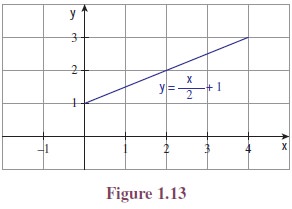
if f : [0, 4] → R is
defined by f(x) = x/2 + 1, then we can plot
the points (x, x/2 + 1) for all ∈ [0, 4]. Then
we will get a straight line segment joining (0, 1) and (4, 3).
(See Figure 1.13)
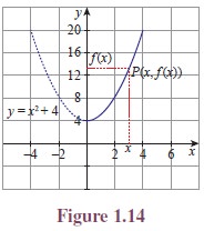
Consider another function f(x) = x2 +
4, x ≥ 0. The function will be given by its
graph. (See Figure 1.14)
Let x be a point in the domain. Let us draw a
vertical line through the point x. Let it meet the curve at P . The point at which the horizontal line drawn
through P meets the y-axis is f(x).
Similarly using horizontal lines through a point y in the
co-domain, we can find the pre-images of y.
Can we say that any curve drawn on the plane be considered as a
function from a subset of R to R? No, we cannot. There is a
simple test to find this.
VERTICAL LINE TEST
As we noted earlier, the vertical line through any
point x in
the domain meets the curve at some point, then the y-coordinate of the point
is f(x). If the vertical line through
a point x in
the domain meets the curve at more than one point, we will get more than one
value for f(x) for one x. This is not allowed in a
function. Further, if the vertical line through a point x in the domain does not
meet the curve, then there will be no image for x; this is also not possible in
a function. So we can say,
“if the vertical line through a
point x in
the domain meets the curve at more than one point or does not meet the curve,
then the curve will not represent a function”.

The curve indicated in Figure 1.15 does not represent a function
from [0, 4] to R because a vertical line meets
the curve at more than one point (See Figure 1.17). The curve indicated in
Figure 1.16 does not represent a function from [0, 4] to R because
a vertical line drawn through x = 2.5 in [0, 4] does
not meet the curve (See Figure 1.18).
Testing whether a given curve represents a function or not by
drawing vertical lines is called vertical line test or
simply vertical test.
2. SOME
ELEMENTARY FUNCTIONS
Some frequently used functions are known by names. Let us list
some of them.
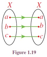
(i) Let X be any
non-empty set. The function f : X → X defined
by f(x) = x for all x ∈ X is called
the identity function on X (See
Figure 1.19). It is denoted by IX or I.
(ii)
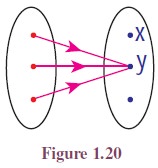
Let X and Y be two sets. Let c be
a fixed element of Y . The
function f : X → Y defined
by f(x) = c for all x ∈ X is
called a constant function (See
Figure 1.20).
The value of a constant function is same for all values of x throughout
the domain.
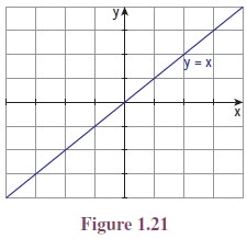
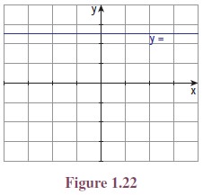
If X and Y are R, then
the graph of the identity function and a constant function are as in Figures
1.21 and 1.22. If X is any set, then the constant function
defined by f(x) = 0 for all x is called
the zero function.
So zero function is a particular case of constant function.
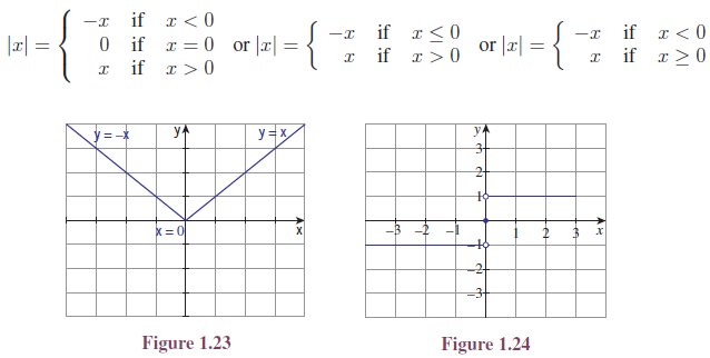
(iii)
The function f : R → R defined
by f(x) = |x|, where |x| is the
modulus or absolute value of x, is called the modulus
function or absolute
value function. (See Figure 1.23.)
Let us recall that |x| is defined as
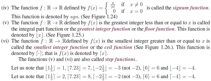
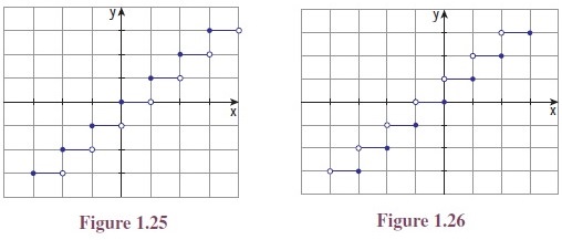
One may note the relations among the names of these functions,
the symbols denoting the functions and the commonly used words ceiling and
floor of a room and their graphs are given in Figures 1.25 and 1.26.
3. Types of
Functions
Though functions can be classified into various types according
to the need, we are going to concentrate on two basic types: one-to-one
functions and onto functions.

Let us look at the two simple functions given in Figure 1.27 and
Figure 1.28. In the first function two elements of the domain, b and c, are mapped into the same
element y,
whereas it is not the case in the Figure 1.28. Functions like the second one
are examples of one-to-one functions.
Let us look at the two functions given in Figures 1.28 and 1.29.
In Figure 1.28 the element z in
the co-domain has no pre-image, whereas it is not the case in Figure 1.29.
Functions like in Figure 1.29 are example of onto functions. Now we define
one-to-one and onto functions.
Let's consider one of the simpler types of
functions that you've graphed; namely, quadratic functions and their associated
parabolas.
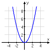
When you first started graphing quadratics,
you started with the basic quadratic:
f (x)
= x2:
Then you did some related graphs, such as:
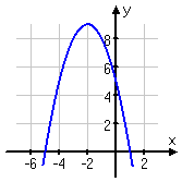
g(x) = –x2 –
4x + 5:
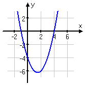
h(x) = x2 – 3x – 4:
k(x) = (x +
4)2:
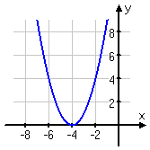
In each of these cases, the basic parabolic shape
was the same. The only difference was where the vertex was, and whether it was
right-side up or upside-down.
If you've been doing your graphing by hand, you've
probably started noticing some relationships between the equations and the
graphs. The topic of function transformation makes these relationships more
explicit.
Moving
up and down
Let's start with the function
notation for the basic quadratic:
f (x) = x2
A function transformation takes whatever is the basic function f (x) and then "transforms" it (or "translates" it),
which is a fancy way of saying that you change the formula a bit and thereby
move the graph around.
For instance, the graph for y = x2 + 3 looks like
this:
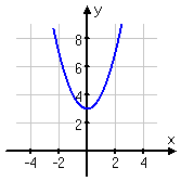
This is three units higher than the basic quadratic, f (x) = x2. That is, x2 + 3 is f (x) + 3. We added a
"3" outside the basic squaring function f (x) = x2 and thereby
went from the basic quadratic x2 to the
transformed function x2 + 3.
This is always true: To move a function up, you add outside the
function: f (x) + b is f (x) moved
up b units. Moving the function down
works the same way; f (x) – b is f (x) moved
down b units.
·
Given g(x) = 4x – 3, what
function h(x) would
represent a downward shift by two units?
Since the original function is being shifted downward by two units, then
the new function is the old one, with a "minus two" tacked onto the
end:
g(x) – 2 = (4x – 3) – 2
= 4x – 5
Then the new function is:
h(x) = 4x – 5
Moving
left and right
On the other hand, y = (x + 3)2 looks like this:
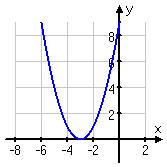
In this graph, f (x) has been
moved over three units to the left: f (x + 3)
= (x + 3)2 is f (x) shifted
three units to the left.
This is always true: To shift a function left, add inside the function's
argument: f (x + b) gives f (x) shifted b units to the left. Shifting to the right works the same way; f (x – b) is f (x) shiftedb units
to the right.
·
Given f (x) = –x2 + 5x + 2, find the expression, in terms of f , for a leftward shift of five units.
To shift the graph side to side, I need to add or subtract inside the
argument of the function (that is, inside the parentheses). To move to the
left, I need (counter-intuitively) to add inside the parentheses. To move five units, I'll
need to add 5 inside the parentheses.
Then my answer is:
f (x +
5)
·
Given s(t)
= 2t + 4, find the expression for the function w(t) which represents a rightward
shift of one unit.
They've told me to shift to the right. To do this, I must
(counter-intuitively) subtract inside the argument. They've told me to shift
rightward by one unit, so I'll be subtracting by 1.
But they haven't told me to express the new function in terms of the
old. They want the actual expression for the rightward shift. So I'll need to
do some algebra, plugging in a "t – 1" for every instance of "t " in the original function. Fortunately,
that function is really simple, so:
w(t) = s(t –
1)
= 2(t –
1) + 4
= 2t – 2 + 4
= 2t +
2
Then my new function is:
w(t) = 2t +
2