PROBABILITY DISTRIBUTIONS
History
The history of random variables and how they
evolved into mapping from sample space to real numbers was a subject of interest.
The modern interpretation certainly occurred after the invention of sets and
maps (1900), but as Eremenko says, random variables were used much earlier.
Mathematicians felt the need to interpret random variables as maps. In 1812,
Laplace published his book on Theory analytique des probabilities in which he
laid down many fundamental results in statistics.

Random Variable
A random variable X is a function defined on a
sample space S into the real numbers R such that the inverse image of points or
subset or interval of R is an event in S, for which probability is assigned.
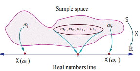
Illustration 1
Suppose a coin is tossed once. The sample space consists of two sample
points H (head) and T (tail).
That is S = { T, H }
Let X : S![]() R be
the number of heads
R be
the number of heads
Then
X(T) = 0 and X(H) = 1
Thus X is a random variable that takes on the
values 0 and 1. If X (ω) denotes the number of heads, then
![]()

Illustration 2
A batch
of 150 students is taken in 4 buses to an excursion. There are 38 students in
the first bus, 36 in second bus, 32 in the third bus, and the remaining
students in the fourth bus. When the buses arrive at the destination, one of
the 150 students is randomly chosen. Suppose that X denotes the number of
students on the bus of that randomly chosen student. Then X takes on the values
32, 36, 38, and 44.
Illustration 3
A coin is
tossed until head occurs.
The
sample space is S = {H,TH,TTH,TTTH,……….}.
Suppose X denotes the number of times the coin
is tossed until head occur.
Then the random variable X takes on
the values 1 2, ,3,……………
Illustration 4
Suppose N is the number of
customers in the queue that arrive at a service desk during a time period, then
the sample space should be the set of non-negative integers. That is S = { 0,
1,2, 3….. } and N is a random variable that takes on the values 0,1,2, 3,…..
Illustration 5
If an
experiment consists in observing the lifetime of an electrical bulb, then a
sample space would be the life time of electrical bulb. Therefore the sample
space is S = [0,![]() . Suppose X denotes the lifetime of the bulb,
then X is a random variable that takes on the values in
. Suppose X denotes the lifetime of the bulb,
then X is a random variable that takes on the values in ![]() .
.
Illustration 6
Let D be
a disk of radius r. Suppose a point is chosen at random in D. Let X denote the
distance of the point from the centre. Then the sample space S = D and X is the
random variable that takes any number from 0 to r. That is ![]()
Types of Random Variable
Discrete random variables
A random variable X is
defined on a sample space S into the real numbers R is called discrete random
variable if the range of X is countable, that is, it can assume only a finite
or countably infinite number of values, where every value in the set S has
positive probability with total one.
Probability Mass Function
If X is a discrete random
variable with discrete values x1,x2,x3,………..
then the function denoted by f (.) or p(.) and defined by
f(xk) = P(X = Xk) , for k = 1,2,3…… is called the probability mass function of X.
Example Two fair
coins are tossed simultaneously (equivalent to a fair coin is tossed twice).
Find the probability mass function for number of heads occurred.
Sol: The sample space S = {H,T}
x {H,T}
That is S = {TT,HT,TH,HH}
Let X be
the random variable denoting the number of heads. Therefore
X(TT) = 0 X(TH) = 1 X(HT) = 1 X(HH) = 2
Then the
random variable X takes on the values 0, 1 and 2

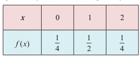
The probabilities are given by
f(0) = P(X = 0) = ![]()
f(1) = P(X = 1) = ![]()
f(2) = P(X = 2) = ![]()
The
function f (x) satisfies the conditions
(i) f(x) ≥ 0 for x = 0,1,2
(ii) ![]() =
= ![]() = f(0) + f(1) + f(2) =
= f(0) + f(1) + f(2) = ![]() = 1
= 1
Therefore f (x) is a probability mass function
given by
Cumulative
Distribution Function or Distribution Function with
probability mass function
The
cumulative distribution function F (x) of a discrete random variable X , taking
the values x1,x2,x3,…. such that x1<x2<x3<……
with probability mass function f(xi)
is F(x) = P(X≤x) = ![]() , x
, x![]() R.
R.
Cumulative
Distribution Function from Probability Mass function
Both the
probability mass function and the cumulative distribution function of a
discrete random variable X contain all the probabilistic information of X. The
probability distribution of X is determined by either of them. In fact, the
distribution function F of a discrete random variable X can be expressed in
terms of the probability mass function f(x) of X and vice versa.
Example - If the probability mass function f (x)
of a random variable X is

Find (i) its cumulative distribution function,
hence find (ii) P (X ≤ 3) and, (iii) P (X ≥ 2)
Solution – P(X<1) = 0 for ![]()
F(1) =
P(X≤1) = P(X<1) + P(X = 1) = 0 + ![]() =
= ![]()
F(2) = P(X≤2) =
P(X<1) + P(X = 1) + P(X = 2) = ![]()
F(3) = P(X<1)
+ P(X = 1) + P(X = 2) + P(X = 3) = ![]()
F(4) = P(X<1)
+ P(X = 1) + P(X = 2) + P(X = 3) + P(X = 4) = ![]()
Therefore the cumulative distribution function is
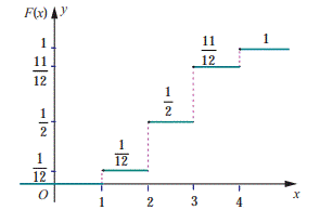
P(X≤3) = F(3) = ![]()
P(X≥2) = 1 – F(1) = 1 -
![]()
Probability
Mass Function from Cumulative Distribution Function
Suppose X is a discrete random variable taking the
values x1,x2,x3,---- such that x1<x2<x3<---- and F(xi) is the distribution
function. Then the probability mass function f(xi) is given by
Example - A
random variable X has the following probability mass function.

Find (i) P(2<X<6) (ii) P(2≤X<5)
(iii) P(X≤4) (iv) P (3<X)
Sol :
Since the given function is a probability mass function, the total
probability is one. That is
k+2k+6k+5k+6k+10k =1
30k = 1
k = ![]()
Therefore the probability mass function is

(i)
P(2<X<6) = f(3) +f(4) + f(5) = ![]()
(ii) P(2≤X<5) = f(2) + f(3)
+f(4) = ![]()
(iii) P(X≤4) = f(1) + f(2) + f(3) +f(4) = ![]() =
= ![]()
(iv) P
(3<X) = f(4) + f(5) + f(6) = ![]() +
+ ![]() =
= ![]()
Continuous
Distributions
Let S be
a sample space and let a random variable X:S![]() R
that takes on any value in a set I of ℝ . Then X is called a continuous random variable
if P(X=x) = 0 for every x in I.
R
that takes on any value in a set I of ℝ . Then X is called a continuous random variable
if P(X=x) = 0 for every x in I.
Probability
density function
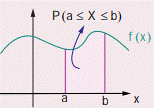
A non-negative real valued
function f (x) is said to be a probability density function if, for each
possible outcome x, x ![]() of a continuous random variable X having the
property
of a continuous random variable X having the
property

Distribution function (Cumulative distribution function)
The distribution function
or cumulative distribution function F (x) of a continuous random variable X
with probability density f(x) is

Distribution function from Probability density function
Both the
probability density function and the cumulative distribution function (or
distribution function) of a continuous random variable X contain all the
probabilistic information of X . The probability distribution of X is
determined by either of them. Let us learn the method to determine the
distribution function F of a continuous random variable X from the probability
density function f (x) of X and vice versa.
Example - If X is the random variable with
probability density function f (x) given by,
f(x) = 
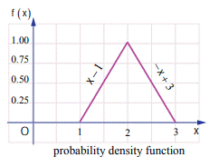
Find the
distribution function F(x).
Sol: By definition, F(x) = P(X ≤ x) = ![]()
When x<1, F(x) =
P(X ≤ x) = ![]() = 0
= 0
When
1≤x<2, F(x)
= P(X ≤ x) = ![]() +
+ ![]() =
= ![]()
When 2≤x<3 F(x) = P(X ≤ x) = ![]() +
+ ![]() +
+ ![]() = 1-
= 1-![]()
When x≥ 3, F(x) = P(X ≤ x) = ![]() +
+ ![]() +
+ ![]() +
+ ![]() = 1
= 1
These give F(x) = 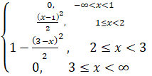
Probability density function from Probability distribution function
Suppose
F (x) is the distribution function of a continuous random variable X . Then the
probability density function f (x)is given by
![]() when ever derivative exists.
when ever derivative exists.
Mathematical Expectation
Suppose X
is a random variable with probability mass (or) density function f (x). The
expected value or mean or mathematical expectation of X , denoted by E (X) or
μ is

Variance
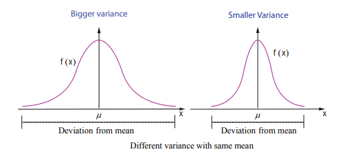
The variance of a random variable X denoted by
Var(X) or V(X) or ![]() (
or
(
or ![]() )
is
)
is
V(X) = E(X-E(X))2
= E(X - µ) 2
·
Square root of variance is called
standard deviation.
Properties of Mathematical expectation and
variance
(i) E(aX+b)
= aE (X) + b , where a and b are
constants
Corollary
1: E (aX) = aE (X) (when b = 0 )
Corollary 2: E (b) = b (when a = 0 )
(ii) Var (X) = E(X2)
- E(X)2
(iii) Var(aX +b) = a2
Var(X) where a and b are constants
Corollary
3: V (aX) = a2 V (X) (when b = 0)
Corollary 4: V (b) = 0 (when a = 0)
Example - Suppose
that f (x) given below represents a probability mass function,

Find (i)
the value of c (ii) Mean and variance.
Sol: (i) ![]()
c2 + 2c2 +
3c2 + 4c2 + c + 2c
= 1
c = ![]()
Hence,
the probability mass function is

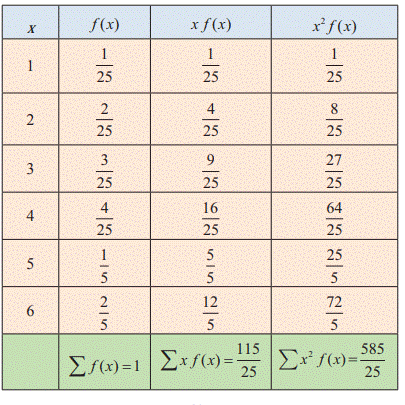
(ii)
To find mean and variance, let us use the following table

Theoretical Distributions: Some Special
Discrete Distributions
The One point
distribution
·
The random variable X has a one
point distribution if there exists a point x0 such that, the
probability mass function f (x) is defined as f (x) = P(X = x0) =1.
·
the mean and the variance are
respectively x0 and 0 .
The Two point distribution
Unsymmetrical Case:
The random variable X has a two point
distribution if there exists two values x1 and x2, such
that
![]()
·
The mean and the variance are respectively
px1 + qx2 and pq(x2 – x1)2
Symmetrical
Case: When p = q = ![]()
The mean and variance
respectively are ![]() and
and ![]()
The Bernoulli
distribution
Let
X be a random variable associated with a Bernoulli trial by defining it as X
(success) = 1 and X (failure) = 0, such that
![]()
X is called a Bernoulli random variable
and f (x) is called the Bernoulli distribution.
·
X is a Bernoulli’s random
variable following with parameter p, the mean μ and variance σ2
of Bernoulli distribution are
µ = p and ![]()
The Binomial Distribution
A
discrete random variable X is called binomial random variable, if X is the
number of successes in n -repeated trials such that
(i)
The n- repeated trials are independent and n is finite
(ii)
Each trial results only two possible outcomes, labelled as ‘success’ or
‘failure’
(iii)
The probability of a success in each trial, denoted as p, remains constant.
·
The binomial random variable X, equals the number of
successes with probability p for a success and q= 1- p for a failure in
n-independent trials, has a binomial distribution denoted by X![]() B(n, p). The probability mass function of X is
B(n, p). The probability mass function of X is
![]() ,
x = 0,1,2, ………..
,
x = 0,1,2, ………..
·
If X is a binomial random
variable with parameters p and n, the mean μ and variance σ2
of binomial distribution are
µ = np and ![]()
Example
- Find the binomial distribution function for a fair die is
rolled 10 times and X denotes the number of times 4 appeared.
Sol: A fair die is rolled ten times and X
denotes the number of times 4 appeared. X is binomial random variable that
takes on the values 0,1,2,3,……,10 with n = 10 and p = ![]() .
.
Probability of getting a four in a
die is p = ![]() and q = 1 – p =
and q = 1 – p = ![]() .
.
Therefore the binomial
distribution is![]()