Applications of Differential Calculus
The primary objective of differential calculus is to
partition something into smaller parts (infinitesimal parts), in order to
determine how it changes. For this reason today’s differential calculus was earlier
named as infinitesimal calculus.
Meaning of Derivatives
Derivative as slope
Slope or Gradient of a line:
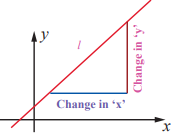
Let l be any given non vertical line as in the figure.
Taking a finite horizontal line segment of any length with the starting point
in the given line l and the vertical line segment starting from the end of the
horizontal line to touch the given line. It can be observed that the ratio of
the vertical length to the horizontal length is always a constant. This ratio
is called the slope of the line l and it is denoted as m .
The slope can be used as a measure to determine the
increasing or decreasing nature of a line. The line is said to be increasing or
decreasing according as m > 0 or m < 0 respectively. When m = 0 , the value of y does not change. Recall that y m= +x c
represents a straight line in the XY plane where m denotes the slope of the
line.
Slope or Gradient of a curve:
Let y = f(x ) be a given
curve. The slope of the line joining the two distinct points (x, f (x)) and the
point (x + h, f (x + h)) is


Example:

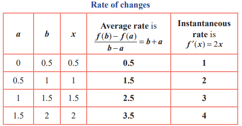
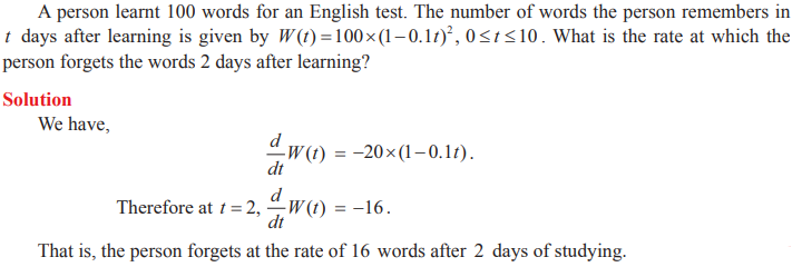
Derivative as rate of change
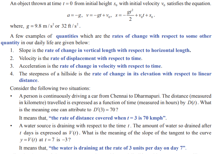
We have seen how the derivative is used to determine
slope. The derivative can also be used to determine the rate of change of one
variable with respect to another. A few examples are population growth rates,
production rates, water flow rates, velocity, and acceleration.
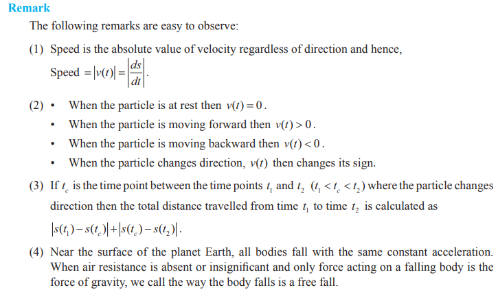
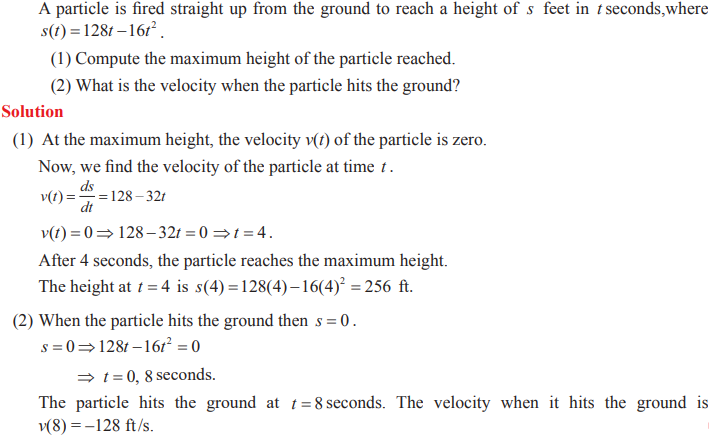
A common use of rate of change is to describe the
motion of an object moving in a straight line. In such problems, it is
customary to use either a horizontal or a vertical line with a designated
origin to represent the line of motion. On such lines, movements in the forward
direction considered to be in the positive direction and movements in the
backward direction is considered to be in the negative direction.

Example
Example
Related rates
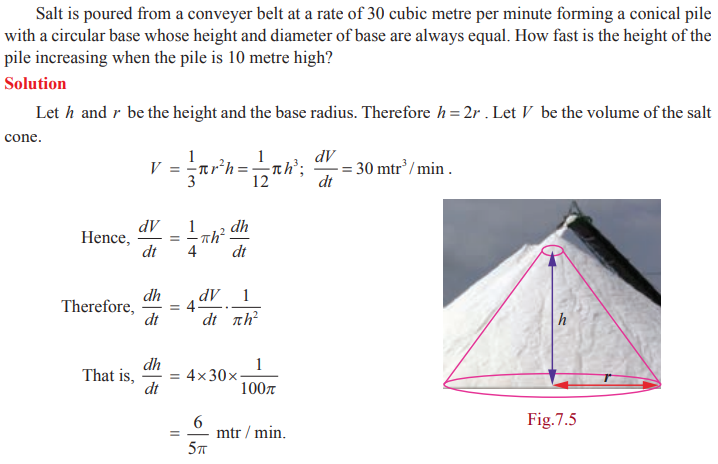
A related rates problem is a problem which involves at
least two changing quantities and asks you to figure out the rate at which one
is changing given sufficient information on all of the others. For instance,
when two vehicles drive in different directions we should be able to deduce the
speed at which they are separating if we know their individual speeds and
directions.
Example
Example
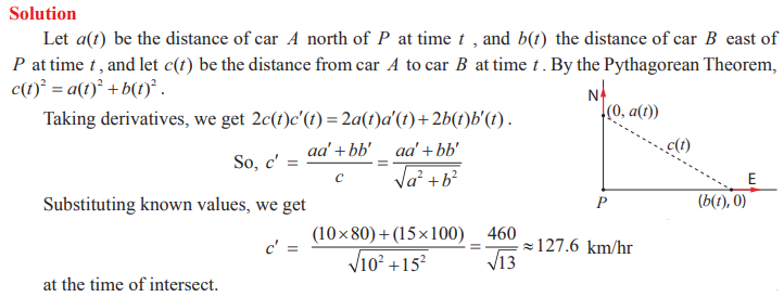
A road running
north to south crosses a road going east to west at the point P . Car A is driving north along the first road, and car B
is driving east along the second road. At a particular time car A i 10 kilometres to the north of P s and traveling at 80
km/hr, while car B is 15 kilometres to the east of P and traveling at 100
km/hr. How fast is the distance between the two cars changing?
Equations of Tangent and Normal
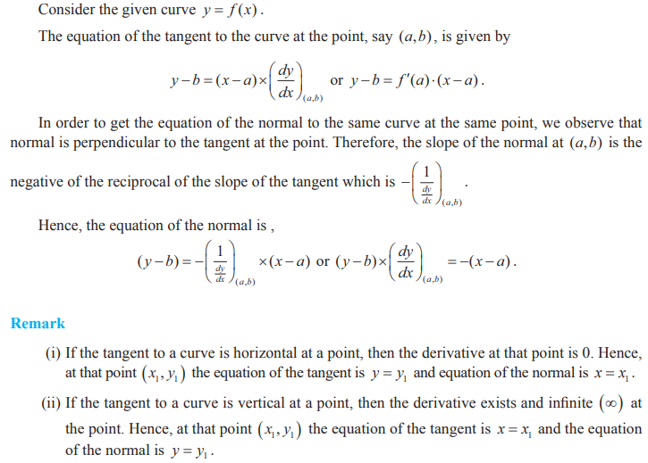
According to Leibniz, tangent is the line through a
pair of very close points on the curve
Definition
1
The tangent line (or simply tangent) to a plane curve
at a given point is the straight line that just touches the curve at that
point.
Definition
2
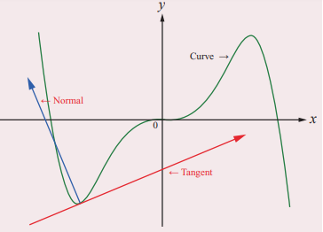
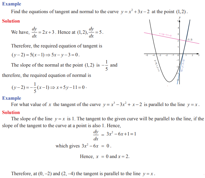
The normal at a point on the curve is the straight
line which is perpendicular to the tangent at that point. The tangent and the
normal of a curve at a point are illustrated in the adjoining figure.
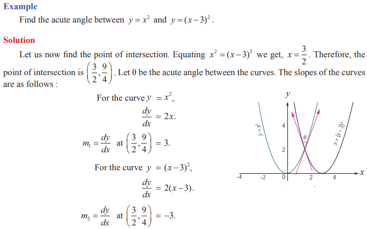
Angle between two curves
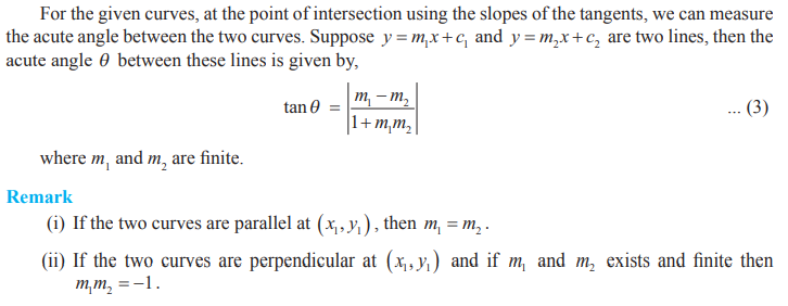
Angle between two curves, if they intersect, is
defined as the acute angle between the tangent lines to those two curves at the
point of intersection.

Mean Value Theorem
Mean value theorem establishes the existence of a
point, in between two points, at which the tangent to the curve is parallel to
the secant joining those two points of the curve. We start this section with
the statement of the intermediate value theorem as follows :

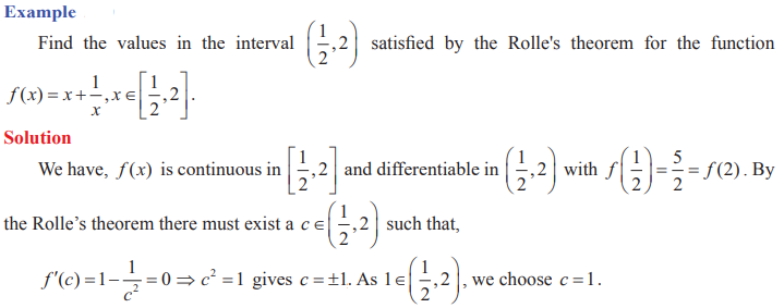
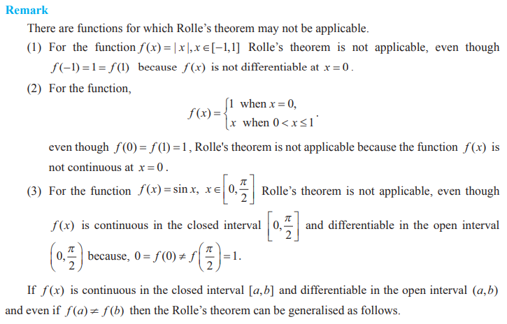
Rolle’s Theorem


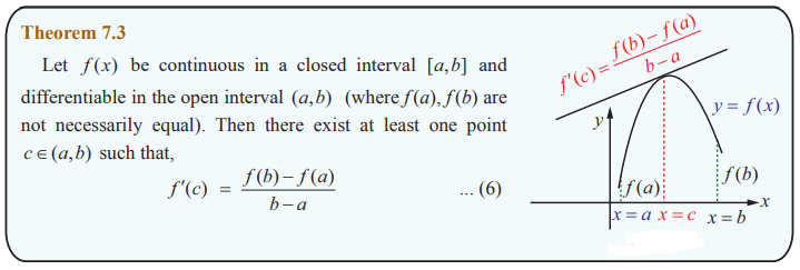
Lagrange’s Mean
Value Theorem
Remark
If f(a) = f(b) then
Lagrange’s Mean Value Theorem gives the Rolle’s theorem. It is also known as
rotated Rolle’s Theorem.

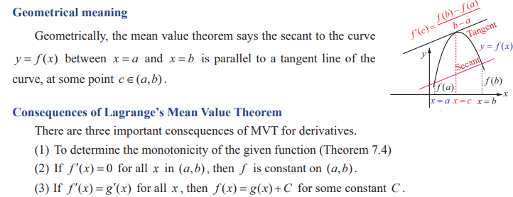
A geometrical meaning of the Lagrange’s mean value
theorem is that the instantaneous rate of change at some interior point is
equal to the average rate of change over the entire interval. This is
illustrated as follows :
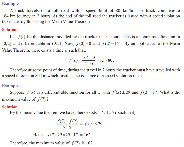
If a car accelerating from zero takes just 8 seconds
to travel 200 m, its average velocity for the 8 second interval is 200/8 = 25
m/s. The Mean Value Theorem says that at some point during the travel the
speedometer must read exactly 90 km/h which is equal to 25 m/s
Application
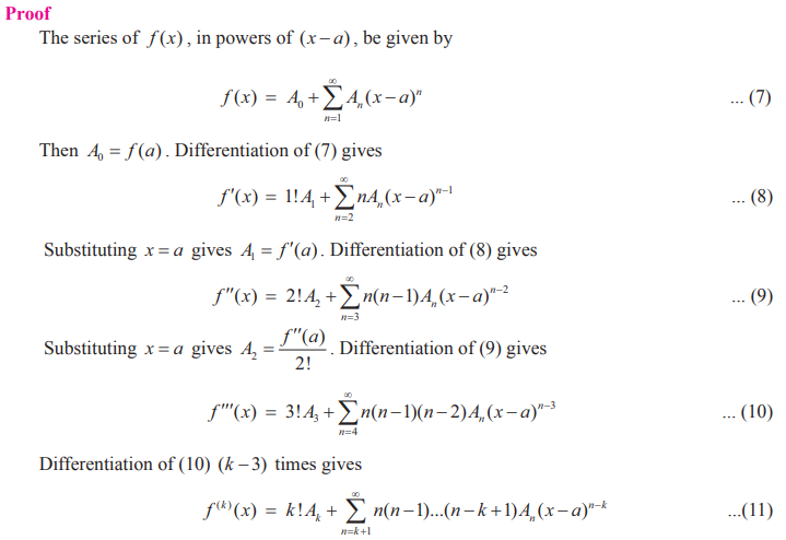
Series Expansions
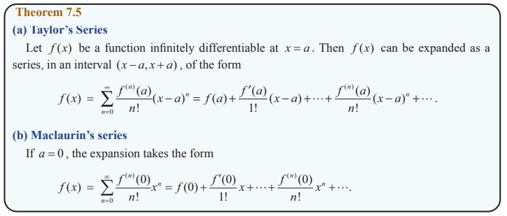
Taylor’s series and Maclaurin's series expansion of a function which are infinitely differentiable.

Indeterminate
Forms
A Limit Process

We say
that they have the form of a number. But values cannot be assigned to them in a
way that is consistent with the usual rules of addition and mutiplication
of numbers. We call these expressions Indeterminate forms. Although they are
not numbers, these indeterminate forms play a useful role in the limiting
behaviour of a function.
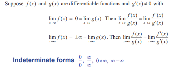
John
(Johann) Bernoulli discovered a rule using derivatives to compute the limits of
fractions whose numerators and denominators both approach zero or ¥. The rule
is known today as l’Hôpital’s Rule (pronounced as Lho pi tal
Rule), named after Guillaume de l’Hospital’s, a
French nobleman who wrote the earliest introductory differential calculus text,
where the rule first appeared in print.
The l’Hôpital’s Rule
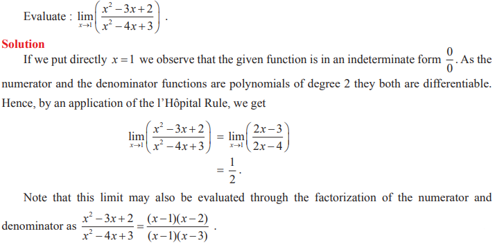
Example
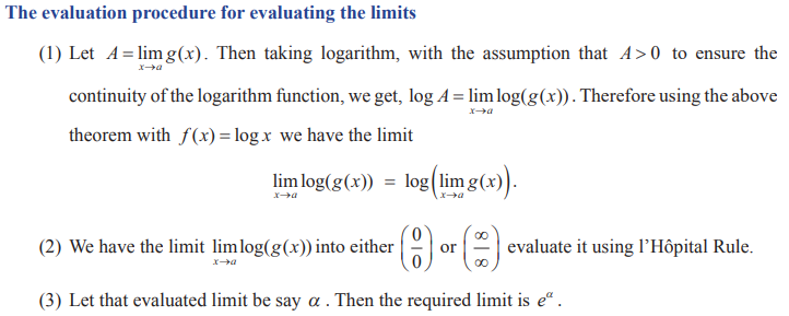
Indeterminate
forms 00, 1∞ and ∞0
In
order to evaluate the indeterminate forms like this, we shall first state the
theorem on the limit of a composite function.

Applications of First Derivative
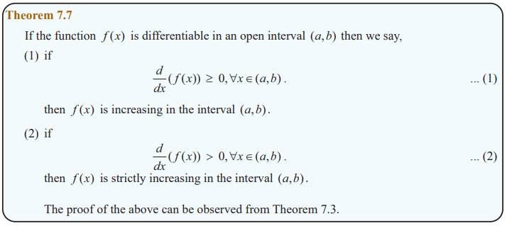
Using the first derivative we can test a function f(x)
for its monotonicity (increasing or decreasing), focusing on a particular point
in its domain and the local extrema (maxima or minima) on a domain.
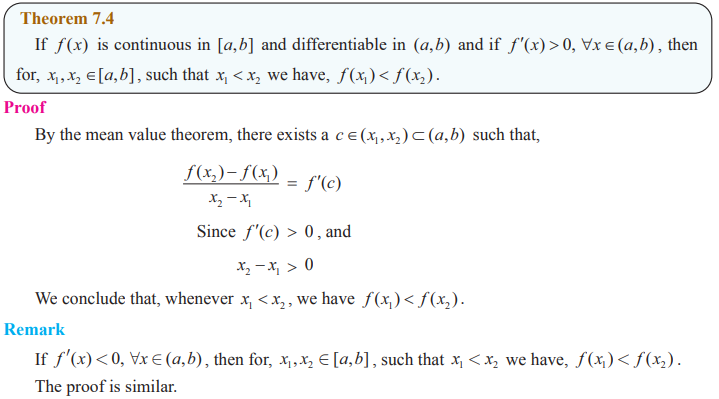
Monotonicity of functions
Monotonicity of functions are its behaviour of
increasing or decreasing

The function f(x) = x is an increasing function in the
entire real line, whereas the function f(x) = −x is a decreasing function
in the entire real line. In general, a given function may be increasing in some
interval and decreasing in some other interval, say for instance, the function
f(x) =|x| is decreasing in (−∞, 0] and is increasing in (0, ∞).
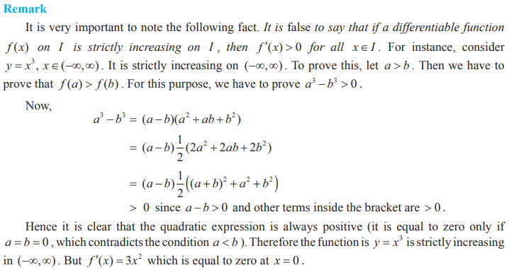
These functions are simple to observe for their monotonicity. But given an
arbitrary function how we determine its monotonicity in an interval of a real
line? That is where following theorem will be useful, which is stated here.


Every stationary point is a critical point however all
critical points need not be stationary points. As an example, the function f (x ) = − | x -17| has a critical point at (17,0 ) but
(17,0 ) is not a stationary point as the function has no derivative at x =17 .
Absolute maxima and minima
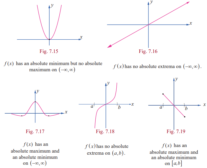
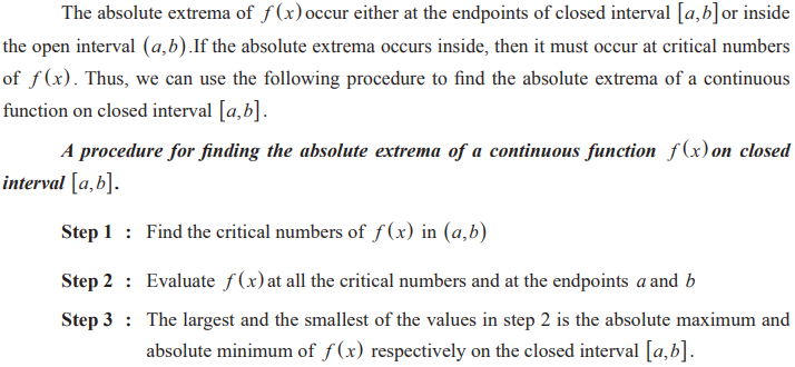
The absolute maxima and absolute minima are referred to describing the largest and smallest values of a function on an interval.

In general, there is no guarantee that a function will
actually have an absolute maximum or absolute minimum on a given interval. The
following figures show that a continuous function may or may not have absolute
maxima or minima on an infinite interval or on a finite open interval.

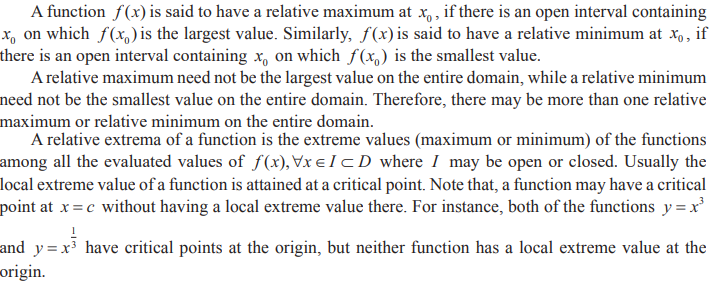
Relative Extrema on an Interval
Extrema using
First Derivative Test
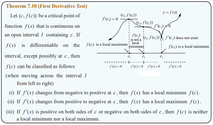
After
we have determined the intervals on which a function is increasing or
decreasing, it is not difficult to locate the relative extrema of the function.
The location or points at which the relative extrema occurs for a given
function f (x ) can be observed through the graph y =
f(x) . However to find the exact point and the value of the extrema of
functions we need to use certain test on functions. One such test is the first
derivative test, which is stated in the following theorem.
Applications
of Second Derivative
Second derivative of a function is used to determine
the concavity, convexity, the points of inflection, and local extrema of
functions.
Concavity, Convexity, and Points of Inflection
A graph is said to be concave down (convex up) at a
point if the tangent line lies above the graph in the vicinity of the point. It
is said to be concave up (convex down) at a point if the tangent line to the
graph at that point lies below the graph in the vicinity of the point. This may
be easily observed from the adjoining graph.


Analytically,
given a differentiable function whose graph y = f(x) ,
then the concavity is given by the following result.

Remark
(1) Any local maximum of a convex upward function
defined on the interval [a,b]
is also its absolute maximum on this interval.
(2) Any local minimum of a convex downward function
defined on the interval [a,b]
is also its absolute minimum on this interval
(3) There is only one absolute maximum (and one
absolute minimum) but there can be more than one local maximum or minimum
Points of Inflection

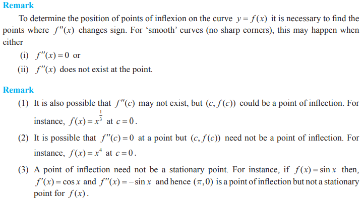
Extrema using Second Derivative Test
The Second Derivative Test: The Second Derivative Test
relates the concepts of critical points, extreme values, and concavity to give a
very useful tool for determining whether a critical point on the graph of a
function is a relative minimum or maximum.

Applications in
Optimization
Optimization
is a process of finding an extreme value (either maximum or minimum) under
certain conditions.
A
procedure for solving for an extremum or optimization problems.
Step 1 : Draw an appropriate figure and label the quantities
relevant to the problem.
Step 2 : Find a experssion for the
quantity to be maximized or minimized.
Step 3 : Using the given conditions of the problem, the quantity
to be extremized .
Step 4 : Determine the interval of possible values for this
variable from the conditions given in the problem.
Step 5 : Using the techniques of extremum (absolute extrimum, first derivative test or second derivative test)
obtain the maximum or minimum.
Symmetry and
Asymptotes
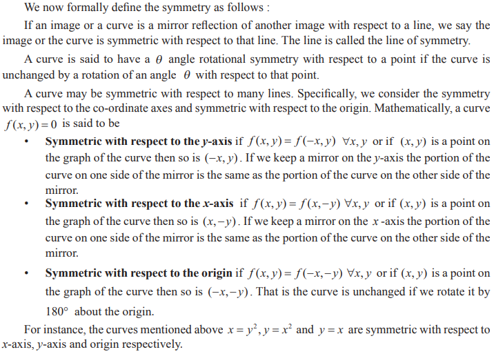
Symmetry
Consider
the following curves and observe that each of them is having some special
properties, called symmetry with respect to a point, with respect to a line.

Asymptotes
An asymptote for the curve y = f(x) is a straight line
which is a tangent at ∞ to the curve. In other words the distance between
the curve and the straight line tends to zero when the points on the curve
approach infinity. There are three types of asymptotes. They are

Sketching of Curves
When we are sketching the graph of functions either by
hand or through any graphing software we cannot show the entire graph. Only a
part of the graph can be sketched. Hence a crucial question is which part of
the curve we need to show and how to decide that part. To decide on this we use
the derivatives of functions. We enlist few guidelines for determining a good
viewing rectangle for the graph of a function. They are :
